$ETH (DAILY): DOWNTREND, yet still BULLISH, losing $4k SUPPORTThe most important chart for CRYPTOCAP:ETH is obviously the DAILY, and it looks like a correction (abc) is was completed on 10/10 when we witnessed a flash-crash to as low as $3450, perfectly in the middle of the SUPPORT ZONE ($3300 - $3600).
After this correction, we should see another surge in price, this would be WAVE 5, the last rally in this cycle, for sure. TARGETS start from $5861 (1.618 fib), and I consider this ELLIOT'S WAVE count to be a clean one, which means, more likely to materialize.
For now, it's been a struggle to stay above the key support/resistance level of $4k, still a DOWNTREND with a recent LOWER LOW followed by a sideways narrow chop.
200 MA at $3260 and upcurved, still a BULL MARKET coin. I'm on the sidelines until it either closes above $4100 or retraces back down by 10 or even 15%.
ETH v CRYPTOCAP:BTC on the WEEKLY, a rebound from the range bottom last APRIL, topped out in AUGUST at 0.0434, currently retracing to an important 0.0344 level, which MUST be hold to keep this year's momentum. Short-term BULLISH long-term BEARISH in relation to the KING.
💙👽
Contains image

CADJPY FREE SIGNAL|SHORT|
✅CADJPY has tapped into a premium supply zone after sweeping liquidity above previous highs. Smart money shows distribution signs with bearish displacement underway — targeting inefficiency below.
—————————
Entry: 109.230
Stop Loss: 109.610
Take Profit: 108.600
Time Frame: 2H
—————————
SHORT🔥
✅Like and subscribe to never miss a new idea!✅

EUR-JPY Free Signal! Sell!
Hello,Traders!
EURJPY SMC based signal. Price has reacted sharply from a premium supply zone, forming a bearish displacement and potential CHoCH on lower timeframes. Expecting a move into discount levels as liquidity below the recent equal lows gets targeted.
-------------------
Stop Loss: 177.959
Take Profit: 177.510
Entry: 177.744
Time Frame: 3H
-------------------
Sell!
Comment and subscribe to help us grow!
Check out other forecasts below too!
Disclosure: I am part of Trade Nation's Influencer program and receive a monthly fee for using their TradingView charts in my analysis.

BMTLSE:BMT is a solid and relatively new project with tech that’s already seeing strong adoption. The chart shows a clean descending wedge pattern forming, signaling potential reversal. From the current price, the setup offers around 200% upside if the breakout confirms.

Accumulation / Distribution King of Crypto has some juice left Monthly; it's in the accumulation peak ranges that the parabolic action occurs. While the accumulation /distribution indicator hovers here, I'm more inclined to lean on the Q4 November-December run. When is the cycle at risk of turning into distribution and the mark-down? When we have the first break under the accumulation peak lows. Our accumulation peak lows were in March of this year. I chose that one as it is the post-halving year accumulation/distribution lows, aligning with the 4-year cycle. So, despite the beating that we've taken, we're still poised for the Q4 November-December run.

The New Trading Era: From Machine Intelligence to Human EdgeThe Oracle That Doesn’t Think but Mirrors
Everyone’s talking about the “rise of artificial intelligence” in trading, algorithms replacing traders, neural networks predicting the next move, machines that seem to think.
But the most extraordinary thing about machine intelligence isn’t its brilliance. It’s its astonishing ability to mirror, to absorb vast amounts of past data and recreate patterns it has already seen. A gigantic echo chamber of past realities.
In other words, what we call “intelligence” in these systems is not understanding, it’s reproduction. They don’t reason; they recognize. They don’t imagine; they approximate.
And yet, that ability to reflect a million past environments can feel almost magical, especially when it responds with coherence that seems human.
But here’s the quiet paradox: one the industry rarely talks about: What we’re witnessing isn’t a new form of intelligence; it’s a new kind of mirror, one that reveals how little we truly understand about our own decision-making.
When Machines Need to Learn the Market Every Day
For most of us, our first real encounter with AI came through models like ChatGPT, tools that belong to a specific subgroup of machine learning known as Large Language Models (LLMs), designed to simulate human-like conversation. That’s where our perception of AI as “brilliant and almost magical” was born. LLMs seem capable of answering anything, from trivial questions to complex reasoning.
Their power, however, doesn’t come from understanding the world. It comes from an extraordinary ability to predict language, a task that, despite its apparent complexity, is remarkably stable and mathematically manageable. The rest is simply scale: access to a massive database of accumulated knowledge, allowing the model not only to predict the next word but also to recreate an entire response by recognizing and recombining patterns it has already seen a million times before.
To understand this better, think of your phone’s autocomplete as a miniature version of ChatGPT, it guesses your next word based on your previous conversations. In such a stable environment, consistency is easy. That’s why language models achieve such high accuracy: their elevated “win rate” comes from playing a game where the rules rarely change.
They may look brilliant, but it’s better to say they’re simply hard-working machines in a stable world.
Trading, however, exists on the opposite side of the spectrum. It lives in a non-stationary world, one where the rules constantly evolve. Today’s conditions will be different tomorrow. Or in five minutes. Or in five seconds. No one knows when or how the shift will happen.
Here lies the crucial difference: a model that “understands” English doesn’t need to relearn grammar every week. A model that trades must relearn market reality every day.
Machine learning thrives on repetition. Markets thrive on surprise.
The Real Disruption: Human Understanding + Machine Power
By truly understanding the capabilities and limitations of machine learning in trading or more broadly, artificial intelligence, we realize that the future isn’t about removing humans from the equation. It lies in understanding how machine power compounds in the right hands.
The next era of trading won’t be about replacing human judgment but amplifying it.
Human contextual reasoning, our ability to interpret uncertainty, adapt, and make sense of nuance, can be combined with the machine’s immense capacity for data processing and execution.
Machines bring speed, scale, and memory. Humans bring intuition, flexibility, and judgment.
The synergy happens when both play their part: the trader designs the logic; the machine executes it flawlessly.
Machines cannot think, but they can learn, replicate, and act at a scale humans simply can’t compete with. When contextual thinking meets computational power, that’s not artificial intelligence, that’s real intelligence.
The trader who treats AI as a tool builds an edge. The one who treats it as an oracle builds a trap.
A Simple Manual for Thinking Right About AI in Trading
Never delegate understanding.
Let the machine calculate, but you must know why it acts. You can outsource the coding of a model, but never the architecture of your trading logic. The logic, the “why,” must remain human.
The basics still apply.
Machine learning doesn’t replace the foundations of trading, it only amplifies them. Risk management, diversification, position sizing, and discipline remain non-negotiable. A model can process data faster than you ever could, but it can’t understand exposure, capital allocation, or your personal tolerance for risk. Those are still your job.
Stay probabilistic.
The use of ML in trading doesn’t erase the hardest lesson of all: predicting prices is a false premise. The right question isn’t “Where will the market go?” but “How should I respond to what it does?” Now imagine the power of machine intelligence working within that probabilistic framework: a system designed to maximize your account’s expected value, not to guess Bitcoin’s price next month. That’s where the real explosion of potential lies.
Build systems that can evolve.
The future won’t belong to the trader with the smartest model, but to the one with the most adaptive one. And remember, you must be the most adaptive asset in your system. Markets evolve; your models must too. There’s no such thing as “build once and deploy forever.” In trading, anything that stops learning starts dying.
From the Illusion of Machine Intelligence to the Power of Human-Driven ML
Machine intelligence isn’t a new oracle, it’s a new instrument. In the wrong hands, it’s noise. In the right hands, it’s leverage. It can multiply insight, scale execution, and compound returns, but only when driven by an intelligent trader who understands its limits.
The trader understands, the machine executes. The trader teaches the machine; the latter amplifies the former’s reach.
In the end, it’s never the algorithm that wins, it’s the human who knows how to use it. And when both work together, one thinking, one learning, that’s not artificial intelligence anymore.
That’s compounded intelligence.
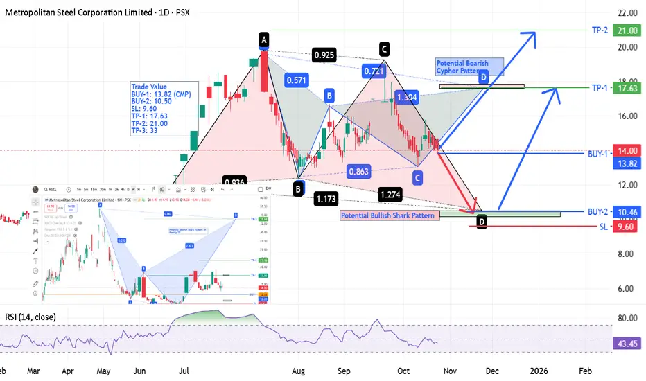
MSCL - PSX - Technical AnalysisOn weekly TF, based on Bearish Shark Harmonic Pattern, the target price is expected to be 30~33 zone by mid Sep 2026.
On Daily TF, two harmonic patterns have been drawn. Red is Bullish Shark Harmonic Pattern whose potential target is 10.46; and other is Bearish Cypher Harmonic Pattern whose target is 17.63.
Suggested Trade Values are:-
BUY-1: 13.82 (CMP)
BUY-2: 10.50
SL: 9.60
TP-1: 17.63
TP-2: 21.00
TP-3: 33
Global Market Time Zone ArbitrageIntroduction
In the increasingly interconnected world of finance, the concept of time zone arbitrage has become a significant factor shaping global market dynamics. As financial markets across continents operate in different time zones, differences in market closing times, liquidity conditions, and price discovery processes create unique opportunities for investors and traders. This temporal gap between global exchanges allows for price discrepancies, which can be exploited through a strategy known as global market time zone arbitrage.
Time zone arbitrage leverages the fact that while one market closes, another opens. For instance, Asian markets like Tokyo or Hong Kong open long before Europe and the United States. This allows traders to act on price movements in one region before another market reacts to the same information, creating both profit opportunities and risks.
This essay explores the concept of global market time zone arbitrage, how it works, its types, real-world examples, associated risks, and the overall impact it has on global financial markets.
Understanding Time Zone Arbitrage
At its core, arbitrage means profiting from price differences of the same asset in different markets or forms. Time zone arbitrage, specifically, involves exploiting these differences that arise because of the time separation between trading sessions across global financial centers such as New York, London, Tokyo, and Sydney.
For example, suppose the Japanese stock market reacts positively to an earnings report of a multinational corporation that is also listed in the U.S. When the Japanese market closes, the U.S. market may not have yet opened. In this time gap, traders can anticipate that U.S. investors will react similarly and buy the stock or related derivatives before the U.S. market adjusts, earning a profit once prices align.
Thus, time zone arbitrage is not just about price differences between markets but also about timing, information flow, and investor reaction across geographies.
Global Financial Market Time Zones
To understand how time zone arbitrage operates, it’s essential to look at the sequence of global market hours:
Asia-Pacific Session: Tokyo, Hong Kong, Singapore, Sydney
European Session: London, Frankfurt, Paris
American Session: New York, Chicago, Toronto
These trading sessions overlap partially—such as the London-New York overlap—where most global liquidity is concentrated. However, outside these overlaps, market isolation creates pricing inefficiencies that form the basis for arbitrage opportunities.
For instance, when the U.S. markets close, Asian traders analyze U.S. closing data overnight and adjust their own markets the following morning. Conversely, European and U.S. traders later react to Asian developments, perpetuating a continuous cycle of price discovery across time zones.
Mechanisms of Time Zone Arbitrage
Time zone arbitrage typically occurs through the following mechanisms:
Information Lag Arbitrage
When significant news or data is released after a market closes, traders in another time zone can act on that information before the first market reopens. For example, if the Federal Reserve announces an unexpected interest rate cut after U.S. markets close, Asian traders can buy Asian equities or currencies that will benefit from a weaker dollar before U.S. investors can respond.
ETF and NAV Timing Mismatches
One of the most well-known forms of time zone arbitrage occurs in mutual funds and exchange-traded funds (ETFs) that hold international assets. These funds’ net asset value (NAV) is calculated based on closing prices of foreign securities, which may be stale by the time U.S. investors trade them. Arbitrageurs exploit this stale pricing by buying or selling fund shares based on information that emerged after the underlying markets closed.
Cross-listing Arbitrage
Many global corporations are listed on multiple stock exchanges (e.g., HSBC in London and Hong Kong). If the stock moves in one market while the other is closed, arbitrageurs can anticipate the direction of the price adjustment once the second market opens.
Currency and Futures Arbitrage
Currencies trade 24 hours, but equity and bond markets do not. Traders may use currency or futures positions to exploit expected movements in markets that have yet to open. For instance, a trader may short yen futures if they expect Japanese equities to fall following negative news in the U.S.
Example: U.S.-Japan Time Zone Arbitrage
A practical example involves the relationship between U.S. and Japanese markets. Suppose Apple Inc. reports outstanding quarterly results after the U.S. markets close. While U.S. investors cannot immediately trade Apple shares, Japanese traders can anticipate a positive impact on Apple’s Japanese suppliers (e.g., Sony, Murata Manufacturing). They buy those stocks during Tokyo’s trading hours, leading to a rise in prices before U.S. investors react the next day.
When the U.S. market opens, Apple’s stock jumps, confirming the arbitrageur’s expectation. The trader profits from the time lag between markets by leveraging cross-market relationships and predictive linkages.
Mutual Fund Timing Arbitrage
A historically significant form of time zone arbitrage occurred in U.S. mutual funds investing in international markets. Because international markets close before U.S. markets, mutual fund NAVs often reflected outdated prices. For example, if Asian markets closed before a rally in U.S. stocks, the NAV of an Asia-focused U.S. mutual fund might remain artificially low. Traders could buy fund shares before the NAV updated and sell them the next day after the price adjustment.
This practice became controversial in the early 2000s, leading to regulatory scrutiny. The 2003 mutual fund scandal in the U.S. revealed that some hedge funds exploited these stale prices systematically, prompting the SEC to enforce stricter pricing mechanisms known as “fair value pricing”, which adjusts foreign security prices to account for time-zone effects.
Types of Time Zone Arbitrage Strategies
Equity Market Arbitrage
Traders use historical correlations between markets (e.g., S&P 500 and Nikkei 225) to predict movements and position themselves accordingly.
Currency and Index Futures Arbitrage
Currency markets react instantly to news. Traders use FX movements as a proxy to predict equity market openings in other regions.
Commodity Market Arbitrage
Commodities such as oil and gold trade globally, but not every derivative market is open simultaneously. Traders may exploit time gaps between futures contracts traded in London, New York, and Shanghai.
ETF and Mutual Fund Arbitrage
Investors trade global ETFs based on anticipated movements in underlying assets, taking advantage of time lags in NAV updates.
Technological Advancements and Algorithmic Arbitrage
With the rise of algorithmic trading and artificial intelligence, time zone arbitrage has evolved beyond manual exploitation of price lags. Advanced trading algorithms now continuously monitor global markets, news feeds, and cross-asset correlations to identify arbitrage opportunities within milliseconds.
These systems use machine learning models to predict how markets will react to global events and execute trades automatically. The speed advantage of these algorithms minimizes human error and maximizes profit capture before prices adjust across time zones.
High-frequency trading (HFT) firms and global hedge funds have particularly benefited from this technological evolution, making time zone arbitrage more efficient and less accessible to retail traders.
Risks Involved in Time Zone Arbitrage
While the concept of arbitrage implies risk-free profit, time zone arbitrage involves several risks due to global uncertainty and information dynamics:
Information Risk
News may be interpreted differently by investors in different regions, leading to unexpected market reactions.
Liquidity Risk
During off-peak hours or illiquid sessions (like pre-market or after-hours trading), executing large trades can cause slippage.
Currency Risk
Exchange rate fluctuations can erode arbitrage profits, especially for cross-border trades involving multiple currencies.
Regulatory Risk
Many regulators, especially in the U.S. and EU, have tightened rules around cross-time-zone and stale-price trading to prevent unfair practices.
Execution and Timing Risk
Delays in order execution or incorrect assumptions about market reactions can quickly turn profits into losses.
Correlation Breakdown
Historical market correlations may not hold during crises or volatility spikes, reducing the predictability of price movements.
Regulatory and Ethical Considerations
Time zone arbitrage often lies in a gray area of financial ethics. While arbitrage itself is legal and contributes to market efficiency, exploiting time-zone pricing inefficiencies in mutual funds was considered unfair to long-term investors. Regulatory bodies like the U.S. Securities and Exchange Commission (SEC) and the Financial Conduct Authority (FCA) have implemented measures such as:
Fair Value Pricing: Adjusting NAVs to reflect real-time global developments.
Time-Stamps on Orders: Preventing late trading after market close.
Enhanced Disclosure: Requiring funds to reveal their valuation methodologies.
These reforms have significantly reduced illicit arbitrage opportunities but have not eliminated legitimate global time zone trading strategies.
Economic Implications of Time Zone Arbitrage
Improved Market Efficiency
Arbitrage helps align prices across global markets, ensuring that information is reflected more quickly and accurately.
Enhanced Liquidity
Continuous trading activity across time zones contributes to global liquidity and reduces bid-ask spreads.
Integration of Global Markets
Time zone arbitrage contributes to tighter linkages between financial centers, reinforcing the idea of a truly “24-hour global market.”
Volatility Transmission
On the downside, arbitrage accelerates the spread of shocks from one region to another, increasing global market interdependence.
Technological Advancement
The pursuit of arbitrage efficiency has driven innovation in trading infrastructure, from algorithmic execution systems to cross-border clearing networks.
Real-World Examples
Asian Market Reaction to U.S. Earnings
Japanese and Hong Kong markets often react first to overnight U.S. corporate earnings, providing early signals for European investors.
Oil Price Arbitrage between London and New York
Crude oil futures listed on ICE (London) and NYMEX (New York) often show short-term discrepancies due to non-overlapping hours, which traders exploit.
ETF Mispricing in Global Funds
U.S.-listed ETFs tracking Asian or European markets often trade at premiums or discounts relative to their NAVs during U.S. hours, offering arbitrage opportunities to institutional traders.
The Future of Time Zone Arbitrage
As globalization deepens and trading technology advances, time zone arbitrage will continue to evolve. The advent of 24-hour trading for certain instruments, such as major stock index futures and cryptocurrencies, is gradually reducing traditional arbitrage windows. However, human behavior, regulatory boundaries, and data asymmetry ensure that time-based inefficiencies will persist to some degree.
The next phase of time zone arbitrage will likely involve AI-driven predictive analytics, capable of modeling how markets in one region will react to developments elsewhere before the markets even open. Quantum computing and blockchain-based global exchanges could further compress time differences, bringing markets closer to real-time synchronization.
Conclusion
Global market time zone arbitrage is a sophisticated strategy that thrives on the natural time differences between global trading hubs. By exploiting price inefficiencies and information lags, traders contribute to global price discovery and market integration. However, this strategy also carries significant risks and ethical considerations, requiring a balance between innovation and regulation.
As global markets continue to move toward seamless 24-hour trading, the opportunities for traditional time zone arbitrage may narrow, but the underlying principle—profiting from the misalignment of time, price, and information—will remain central to the mechanics of global finance.
Developed Market and Emerging MarketIntroduction
The global economy is an interconnected network of nations at different stages of economic development. These stages are generally categorized into developed markets, emerging markets, and frontier markets. Among them, developed and emerging markets play the most significant roles in shaping international trade, investment flows, and financial stability. Understanding these two categories is essential for investors, policymakers, and economists who analyze global financial dynamics, risk profiles, and growth opportunities.
Developed markets represent mature, advanced economies with strong industrial bases, high income per capita, and stable political systems. Emerging markets, on the other hand, are countries in the process of industrialization and modernization, showing rapid growth but also facing economic volatility and structural challenges. This distinction helps investors gauge risk, return potential, and diversification strategies in global portfolios.
1. Definition and Concept
Developed Market
A developed market (also known as an advanced or mature market) refers to a country with a highly industrialized economy, well-established financial systems, and high living standards. These nations have robust infrastructure, sophisticated regulatory frameworks, and stable political environments that promote predictable business operations. Their economic activities are primarily driven by services and advanced manufacturing rather than agriculture or basic industries.
International organizations such as the International Monetary Fund (IMF), World Bank, and United Nations classify developed markets based on indicators like:
Gross Domestic Product (GDP) per capita
Human Development Index (HDI)
Financial market sophistication
Industrial diversification
Institutional strength and governance quality
Examples of developed markets include:
United States
Canada
United Kingdom
Germany
France
Japan
Australia
South Korea
Switzerland
These economies form the backbone of global financial systems and often host major stock exchanges such as the NYSE, NASDAQ, London Stock Exchange, and Tokyo Stock Exchange.
Emerging Market
An emerging market is a nation transitioning from a developing to a developed economy. These countries experience rapid industrialization, urbanization, and integration into the global economy, leading to substantial growth potential. However, they also face higher risks, including political instability, inflation volatility, and weaker institutional frameworks.
The term "emerging market" was popularized by economist Antoine van Agtmael in the 1980s to describe countries with growing capital markets that were becoming attractive to foreign investors.
Criteria defining emerging markets include:
Moderate to high GDP growth rates
Expanding middle class
Increasing foreign investment
Developing infrastructure and technology
Improving governance and market reforms
Prominent emerging markets include:
China
India
Brazil
Russia
Mexico
Indonesia
South Africa
Turkey
Thailand
These countries often form part of groupings such as BRICS (Brazil, Russia, India, China, South Africa) or MINT (Mexico, Indonesia, Nigeria, Turkey).
2. Key Characteristics
Developed Markets
High Income Levels:
Developed economies have high GDP per capita, reflecting widespread wealth and purchasing power. For example, countries like the U.S. and Switzerland boast per capita incomes exceeding $60,000 annually.
Mature Financial Systems:
Their banking systems, capital markets, and insurance sectors are well-established and transparent, governed by strong regulatory frameworks.
Low Political and Economic Risk:
Stable governments, rule of law, and consistent economic policies create confidence among investors.
Advanced Infrastructure:
Efficient transportation, communication, and energy networks support productivity and competitiveness.
Technological Leadership:
Developed nations are at the forefront of innovation in industries such as IT, biotechnology, and renewable energy.
Stable Currency and Inflation:
Their central banks, such as the U.S. Federal Reserve or the European Central Bank, maintain price stability and sound monetary policy.
Emerging Markets
High Growth Potential:
Emerging economies often record faster GDP growth, sometimes exceeding 5–8% annually, driven by industrialization and rising domestic consumption.
Expanding Middle Class:
Economic development leads to a growing middle-income population, which boosts demand for goods, housing, and financial services.
Reform-Driven Economies:
Structural reforms, such as privatization and liberalization, make these markets more attractive to foreign investors.
Developing Financial Systems:
Their capital markets are growing but may still lack depth, transparency, and liquidity compared to developed markets.
Currency and Political Volatility:
Exchange rates and government policies can fluctuate significantly, affecting investor confidence.
Urbanization and Industrialization:
Rapid city expansion and manufacturing growth drive job creation and export competitiveness.
3. Economic Indicators Comparison
Indicator Developed Markets Emerging Markets
GDP per capita High (> $40,000) Moderate ($5,000–$20,000)
Growth rate Moderate (1–3%) High (4–8%)
Inflation Low and stable Moderate to high
Infrastructure Advanced Developing
Political stability Strong Varies widely
Currency stability High Often volatile
Industrial base Services and high-tech Manufacturing and agriculture
Income inequality Relatively low Often high
Financial markets Deep and liquid Expanding but less liquid
4. Role in Global Economy
Developed Markets’ Role
Developed economies act as the anchors of global finance and trade. They host the largest multinational corporations, reserve currencies, and financial hubs. The U.S. dollar, euro, and yen serve as international mediums of exchange, influencing global monetary policy. Their advanced financial systems provide capital to the rest of the world through foreign direct investments (FDI) and institutional funds.
They also drive technological innovation and research & development, setting global standards in production and governance. Developed markets’ consumer demand fuels global exports from emerging and developing nations, linking their prosperity to world trade flows.
Emerging Markets’ Role
Emerging economies represent the engine of global growth in the 21st century. They contribute a significant share of global GDP expansion due to large populations, rapid industrialization, and consumption growth. For instance, China and India alone account for over one-third of global economic growth.
They are crucial suppliers of raw materials, manufactured goods, and increasingly digital services. Moreover, they offer investment diversification opportunities, as their growth cycles may differ from developed economies. Emerging markets also play an essential role in addressing global challenges such as energy demand, environmental sustainability, and digital transformation.
5. Investment Perspective
From an investment standpoint, both developed and emerging markets present distinct risk-reward profiles.
Developed Market Investments
Investing in developed economies offers stability, transparency, and lower risk. Their stock markets are highly liquid and regulated, making them ideal for long-term investors seeking steady returns. However, growth opportunities may be limited because of market maturity and slower GDP expansion.
Common investment vehicles include:
Blue-chip equities (e.g., Apple, Microsoft, Nestlé)
Government bonds (e.g., U.S. Treasuries)
Index funds tracking major benchmarks (e.g., S&P 500, FTSE 100)
Emerging Market Investments
Emerging markets provide higher growth potential but also higher volatility. Investors are attracted to the potential for strong returns from sectors like infrastructure, consumer goods, and technology. However, risks include political instability, currency depreciation, and weaker governance.
Investment opportunities include:
Local equities and bonds
Exchange-traded funds (ETFs) tracking emerging indices (e.g., MSCI Emerging Markets Index)
Direct investment in infrastructure or start-ups
Diversifying portfolios across both markets helps balance stability and growth potential.
6. Challenges Faced by Each Market Type
Challenges in Developed Markets
Slow Growth:
Mature economies experience limited GDP expansion due to market saturation and aging populations.
High Debt Levels:
Many developed nations carry large public debts, creating fiscal pressures.
Technological Disruption:
Automation and AI may lead to job displacement and inequality.
Geopolitical Risks:
Trade disputes and policy shifts (e.g., Brexit, U.S.–China tensions) can affect global stability.
Challenges in Emerging Markets
Political Instability:
Government changes and weak institutions can disrupt economic policy.
Inflation and Currency Risk:
Volatile exchange rates can deter foreign investment.
Dependence on Commodities:
Many emerging economies rely heavily on exports like oil or minerals, making them vulnerable to price swings.
Infrastructure Deficits:
Inadequate roads, power supply, and communication networks limit industrial efficiency.
Capital Flight:
When global interest rates rise, investors often withdraw funds from riskier emerging markets.
7. Interdependence Between Developed and Emerging Markets
Globalization has woven developed and emerging markets into a mutually dependent economic fabric. Developed nations invest heavily in emerging markets for higher returns and resource access, while emerging markets rely on developed economies for technology, capital, and demand.
For example:
U.S. and European companies outsource manufacturing to Asia to reduce costs.
China and India import advanced machinery and software from developed countries.
Financial crises or interest rate changes in the U.S. can ripple across emerging economies.
Thus, while they differ in structure and stability, both market types are interlinked in global trade, investment, and policy networks.
8. The Future Outlook
The future of global growth is expected to be driven increasingly by emerging markets. By 2050, countries like China, India, and Indonesia are projected to become the world’s largest economies in purchasing power parity (PPP) terms. Their rising consumer bases, technological adoption, and urbanization will reshape global demand patterns.
However, developed markets will continue to dominate in innovation, finance, and governance standards. They will serve as models of economic stability and sustainability, influencing the global economic architecture through institutions such as the IMF, World Bank, and G7.
The key to a balanced global economy lies in cooperation between developed and emerging markets, focusing on trade fairness, technology transfer, and sustainable development.
Conclusion
Developed and emerging markets represent two distinct yet complementary pillars of the global economic system. Developed markets embody stability, efficiency, and innovation, while emerging markets offer dynamism, growth, and transformation. Together, they shape the rhythm of global finance, trade, and investment.
For investors and policymakers alike, understanding the interplay between these markets is crucial. Developed economies provide safe, predictable environments for steady returns, whereas emerging markets offer the promise of high growth with commensurate risks. As globalization deepens and digital technologies blur traditional boundaries, the collaboration and balance between these two market categories will define the future of global prosperity.
Fluctuation Effects on the Global EconomyIntroduction
The global economy is a dynamic and interconnected system that continuously experiences fluctuations due to various internal and external factors. Economic fluctuations — often referred to as business cycles — involve alternating periods of expansion and contraction in economic activity, influenced by changes in market forces, monetary policies, trade dynamics, technological innovations, and geopolitical developments. These fluctuations impact every aspect of the world economy, including employment levels, inflation rates, investment flows, international trade, and overall economic stability. Understanding how these fluctuations affect the global economy is crucial for investors, policymakers, and businesses seeking to navigate uncertainty and maintain stability.
1. Understanding Economic Fluctuations
Economic fluctuations refer to the unpredictable variations in key macroeconomic indicators such as GDP growth, inflation, interest rates, and employment. These fluctuations are not always harmful; they represent natural movements in response to supply-demand shifts, innovation cycles, and consumer confidence.
1.1 Business Cycles
Business cycles typically include four phases:
Expansion: Characterized by increasing production, employment, and consumer spending.
Peak: The economy operates at full capacity, often leading to inflationary pressures.
Contraction (Recession): Decline in output, demand, and investment, often resulting in job losses.
Trough: The lowest point before recovery begins.
1.2 Causes of Economic Fluctuations
Economic fluctuations are caused by multiple factors:
Monetary and fiscal policy shifts
Commodity price volatility (especially oil and gas)
Technological disruptions
Global trade imbalances
Financial crises and capital flows
Geopolitical tensions
Natural disasters or pandemics
These elements interact in complex ways, creating ripple effects across the world economy.
2. Impact on Global Trade and Investment
One of the most direct consequences of economic fluctuations is their effect on global trade and investment. When major economies experience instability, their trading partners face repercussions as well.
2.1 Trade Volume Volatility
During periods of expansion, demand for imports rises as consumers and industries require more goods and raw materials. Conversely, recessions reduce purchasing power and decrease international trade. For instance, the 2008 global financial crisis caused global trade to contract by nearly 12% in 2009, marking one of the steepest declines in modern history.
2.2 Foreign Direct Investment (FDI)
Fluctuations influence investor confidence. During booms, foreign investors channel funds into emerging markets, seeking higher returns. However, in uncertain times, investors retreat to safe-haven assets like gold, U.S. Treasury bonds, or stable currencies such as the U.S. dollar and Swiss franc. Such movements create capital flight from developing economies, reducing growth potential.
2.3 Exchange Rate Instability
Economic fluctuations often trigger exchange rate volatility. For example, when a country experiences inflation or a balance of payment deficit, its currency value declines. This impacts export competitiveness and import costs, influencing inflation and consumption globally. Exchange rate fluctuations thus act as both a symptom and a catalyst of broader economic cycles.
3. Employment and Income Inequality
Economic fluctuations deeply influence labor markets and income distribution across countries.
3.1 Employment Cycles
In expansionary phases, companies hire more workers to meet rising demand, reducing unemployment and increasing wages. However, recessions often lead to layoffs, wage cuts, and higher job insecurity. Millions of workers globally lost their jobs during the COVID-19 pandemic recession, highlighting how fluctuations can rapidly alter employment landscapes.
3.2 Wage and Income Inequality
Fluctuations tend to worsen income inequality. High-skilled workers and capital owners recover quickly during upturns, while low-skilled laborers face longer unemployment spells. Moreover, automation and digitization, which often accelerate during downturns, can replace labor-intensive jobs, widening wage disparities within and across nations.
4. Inflation, Deflation, and Price Instability
Fluctuations have a direct impact on price stability, which is essential for economic predictability.
4.1 Inflationary Pressures
During economic expansions, strong demand can outpace supply, leading to inflation. Moderate inflation encourages spending and investment, but excessive inflation — like the hyperinflation seen in Zimbabwe or Venezuela — erodes purchasing power and destabilizes the economy.
4.2 Deflationary Risks
Conversely, during recessions, falling demand can cause deflation — a sustained drop in prices. Deflation discourages consumption and investment, as people delay purchases expecting further price falls. Japan’s “Lost Decade” (1991–2001) is a prime example of prolonged deflation stalling economic growth.
4.3 Commodity Price Fluctuations
Oil, gas, metals, and agricultural products often experience sharp price swings. These fluctuations affect both producers and consumers globally. For instance, a sudden spike in oil prices increases transportation and manufacturing costs, leading to inflationary pressures worldwide.
5. Effects on Financial Markets
Financial markets are extremely sensitive to economic fluctuations. Investors continuously adjust their portfolios based on perceived risks and returns.
5.1 Stock Market Volatility
Economic uncertainty increases volatility in global stock indices. During downturns, corporate earnings decline, leading to market sell-offs. For example, the 2020 pandemic crash wiped out trillions in global market capitalization within weeks. Conversely, strong recovery expectations can drive rapid market rallies, as seen in 2021.
5.2 Bond Markets
Interest rate fluctuations, driven by central bank policy responses, affect bond yields. In times of recession, central banks cut rates to stimulate borrowing, pushing bond prices up. During inflationary periods, higher interest rates cause bond prices to fall.
5.3 Currency and Crypto Markets
Exchange rates and digital currencies also reflect economic fluctuations. Investors flock to stable currencies during uncertainty, while risk appetite during recoveries often boosts speculative assets like cryptocurrencies.
6. Policy Responses to Economic Fluctuations
Governments and central banks play crucial roles in mitigating the adverse impacts of economic fluctuations.
6.1 Monetary Policy
Central banks use tools such as interest rate adjustments, quantitative easing (QE), and reserve requirements to stabilize the economy. Lowering rates encourages borrowing and investment during recessions, while raising rates helps control inflation during booms. For instance, during the 2008 financial crisis, the U.S. Federal Reserve implemented QE to inject liquidity and support recovery.
6.2 Fiscal Policy
Governments use spending and taxation to influence economic activity. During downturns, expansionary fiscal policy — such as infrastructure spending and tax cuts — stimulates demand. Conversely, contractionary fiscal measures help control overheating during rapid expansions.
6.3 International Coordination
Because modern economies are interconnected, international institutions like the IMF, World Bank, and G20 play key roles in coordinating responses to global fluctuations. During the COVID-19 crisis, global stimulus packages totaling over $14 trillion were deployed to stabilize financial systems and support recovery.
7. Sectoral Impacts of Fluctuations
Different sectors of the economy respond differently to fluctuations.
7.1 Manufacturing and Trade
Manufacturing and trade sectors are highly sensitive to demand shifts. Recessions reduce exports and industrial production, whereas recovery phases trigger rapid rebounds in supply chains and production.
7.2 Technology and Innovation
Economic uncertainty often accelerates technological innovation, as companies seek efficiency. For example, digital transformation and automation surged during the pandemic as businesses adapted to remote operations.
7.3 Real Estate
Fluctuations impact property values, mortgage rates, and construction activity. Booming economies raise housing prices, while recessions lead to declines in real estate demand and construction investments.
7.4 Energy and Commodities
Commodity-based economies, such as those of Russia, Saudi Arabia, or Brazil, experience strong cyclical effects due to volatile global prices of oil, metals, and agricultural products.
8. Global Inequality and Regional Divergence
Economic fluctuations often exacerbate global inequality. Developed economies typically have stronger institutions, diversified industries, and better fiscal capacity to absorb shocks. In contrast, developing countries rely heavily on exports or commodities, making them more vulnerable to downturns.
8.1 Emerging Markets Vulnerability
When global interest rates rise, emerging markets face capital outflows, currency depreciation, and higher borrowing costs. For example, when the U.S. Federal Reserve tightens policy, many emerging markets experience economic slowdowns.
8.2 Regional Recovery Gaps
The pace of recovery also varies by region. Advanced economies often rebound faster due to stimulus support and technological strength, while low-income nations face delayed recoveries due to limited fiscal space and debt burdens.
9. Psychological and Behavioral Effects
Economic fluctuations also have psychological consequences for consumers and investors.
Consumer Confidence: People spend less when they feel uncertain about the future, deepening recessions.
Investor Sentiment: Fear and speculation drive market volatility. Behavioral biases often cause overreactions to news and policy changes.
Corporate Behavior: Companies may delay expansions, acquisitions, or R&D investments due to uncertainty, affecting long-term innovation and productivity.
10. Future Outlook: Managing Global Economic Fluctuations
As globalization deepens, economic fluctuations are likely to become more interdependent. The future global economy will be influenced by factors such as:
Technological transformation (AI, automation, digital finance)
Climate change and green energy transition
Geopolitical realignments
Debt sustainability and financial regulation
Policymakers must adopt forward-looking strategies, including:
Strengthening financial safety nets
Promoting inclusive growth
Enhancing transparency and international coordination
Diversifying economies to reduce vulnerability to global shocks
The world needs resilient systems that can withstand fluctuations without causing widespread human and economic hardship.
Conclusion
Fluctuations are an inevitable feature of the global economic landscape. While they bring challenges such as unemployment, inflation, and inequality, they also create opportunities for innovation, reform, and structural transformation. The key lies in how nations, institutions, and individuals respond to these changes. Effective policy coordination, sound financial management, and adaptive business strategies can mitigate adverse impacts and harness positive momentum. Ultimately, understanding and managing economic fluctuations is essential for achieving long-term stability, sustainable growth, and global prosperity.

Global Finance Control on Central BanksIntroduction
Central banks are the cornerstone of a nation’s monetary and financial stability. They regulate the money supply, manage interest rates, maintain price stability, and act as lenders of last resort during crises. Examples include the Federal Reserve (U.S.), the European Central Bank (ECB), the Bank of Japan (BoJ), and the Reserve Bank of India (RBI). However, in today’s deeply interconnected global economy, the autonomy of central banks is not absolute. They operate within a global financial system heavily influenced by international capital flows, global trade dynamics, foreign exchange markets, and powerful multinational institutions.
The control of global finance over central banks is a topic of major debate among economists and policymakers. While central banks are officially independent, their actions are shaped by the pressures and movements within global markets. Understanding this interplay is critical to analyzing how global economic policies are formed and how nations maintain financial sovereignty.
1. The Role and Functions of Central Banks
Central banks serve several core functions within national economies:
Monetary Policy Implementation – They regulate interest rates and control money supply to achieve economic stability.
Price Stability and Inflation Control – Ensuring that inflation remains within target levels protects the value of money and public confidence.
Financial Stability and Regulation – Central banks oversee financial institutions to prevent systemic crises.
Foreign Exchange Management – They manage exchange rates, foreign reserves, and currency interventions.
Lender of Last Resort – During financial distress, central banks provide emergency liquidity to banks and financial institutions.
Economic Growth Promotion – By influencing credit availability and investment, central banks indirectly promote growth and employment.
In theory, these functions are carried out independently from political or external influences. However, in the era of globalized finance, maintaining such independence has become increasingly difficult.
2. The Global Financial System and Its Influence
The global financial system is a web of interconnected markets and institutions, including international banks, hedge funds, multinational corporations, and supranational organizations such as the International Monetary Fund (IMF) and World Bank. It is characterized by:
Cross-border capital flows
Global investment funds and currency trading
Interconnected banking networks
International debt and credit markets
Global rating agencies and financial intermediaries
These elements create a financial ecosystem in which no central bank can act in isolation. The decisions made by one major central bank—particularly the U.S. Federal Reserve—can ripple across the globe, influencing exchange rates, asset prices, and borrowing costs in multiple countries.
3. The U.S. Federal Reserve’s Global Dominance
The U.S. dollar is the world’s primary reserve currency, accounting for nearly 60% of global reserves and the majority of international trade settlements. As a result, the Federal Reserve (Fed) exerts substantial indirect control over global financial conditions.
When the Fed changes its interest rates or monetary policy stance, the effects are immediate and widespread:
Emerging markets experience capital inflows or outflows based on the attractiveness of U.S. yields.
Currency values fluctuate as investors shift between the dollar and other currencies.
Global borrowing costs rise or fall depending on U.S. Treasury yields.
For example, the 2013 "Taper Tantrum" occurred when the Fed announced it would reduce its quantitative easing program. This led to a massive outflow of capital from emerging markets, causing currency depreciation and market volatility worldwide. Central banks in countries like India, Brazil, and Indonesia were forced to raise interest rates or intervene in currency markets to stabilize their economies.
Thus, while national central banks manage their domestic economies, their room for maneuver is constrained by decisions made in Washington.
4. The Role of the IMF and World Bank
Institutions such as the International Monetary Fund (IMF) and the World Bank play a central role in influencing the monetary policies of developing and emerging nations. While these institutions provide financial assistance and development loans, their programs often come with policy conditionalities.
For instance, countries seeking IMF loans during balance-of-payment crises are required to implement austerity measures, fiscal discipline, and structural reforms, which often restrict the central bank’s ability to conduct independent monetary policy.
Examples include:
The Asian Financial Crisis (1997–1998), where IMF intervention imposed tight monetary and fiscal controls on countries like Thailand, Indonesia, and South Korea.
Latin American debt crises of the 1980s, where IMF programs demanded strict monetary policies and privatization measures.
Such conditions reflect how global financial institutions can indirectly control the policy framework of central banks, particularly in financially vulnerable nations.
5. Global Capital Flows and Market Pressures
Modern financial markets operate on a 24-hour global cycle, with trillions of dollars moving across borders daily. These massive flows of “hot money” can destabilize currencies and bond markets, forcing central banks to adjust their policies even if they conflict with domestic economic needs.
For instance:
A sudden capital outflow can devalue a country’s currency, raise import costs, and fuel inflation.
To counter this, the central bank may need to raise interest rates, which can slow economic growth.
Conversely, large capital inflows can create asset bubbles and inflationary pressures, requiring monetary tightening.
In this sense, global financial markets act as a disciplinary mechanism, rewarding or punishing central banks based on their policies. Nations with high fiscal deficits or loose monetary policies often face downward pressure on their currency or increased borrowing costs in global bond markets.
6. Exchange Rate Systems and Dependence
Exchange rate management is another area where global finance limits central bank independence. Most countries today operate under floating exchange rates, meaning their currency value is determined by market forces. However, even floating currencies are vulnerable to speculative attacks and global shocks.
Countries that peg their currency to the dollar or euro must align their monetary policies with the anchor currency’s central bank, effectively surrendering policy control.
For example, countries in the Eurozone have ceded national control to the European Central Bank (ECB), which sets a unified monetary policy for 20 diverse economies.
Similarly, economies with dollar pegs, like Hong Kong or Saudi Arabia, must follow U.S. interest rate trends to maintain currency stability.
Thus, through exchange rate mechanisms, global finance exerts control over domestic policy decisions.
7. The Power of Global Financial Institutions and Rating Agencies
Global credit rating agencies such as Moody’s, Standard & Poor’s, and Fitch Ratings have significant influence on national monetary conditions. A downgrade in a country’s sovereign rating can lead to higher borrowing costs, reduced investor confidence, and currency depreciation.
Central banks must often take preemptive actions—such as tightening monetary policy or maintaining high reserves—to maintain favorable credit ratings. This dependence on external validation further diminishes true policy autonomy.
Similarly, international investment banks and hedge funds influence global liquidity conditions. Their collective actions can amplify or counteract central bank policies, shaping market expectations and financial stability.
8. The Challenge of Central Bank Independence
Central bank independence is designed to prevent political interference and maintain policy credibility. However, true independence is a relative concept. Central banks must balance domestic economic objectives with global realities, including:
Exchange rate volatility
Global interest rate movements
Commodity price fluctuations
Investor sentiment and risk appetite
For smaller or developing economies, these external pressures can severely constrain policy options. Even advanced economies are not immune—consider the European Central Bank, which must balance the interests of both strong economies like Germany and weaker ones like Greece or Italy.
9. Global Crises and Central Bank Coordination
During periods of global crisis, such as the 2008 Global Financial Crisis or the COVID-19 pandemic, central banks often act in coordination. The Federal Reserve, ECB, Bank of Japan, and others engaged in synchronized interest rate cuts and quantitative easing programs to inject liquidity into global markets.
While such cooperation stabilized financial systems, it also highlighted the growing interdependence of global central banks. The Fed’s swap lines—temporary currency exchanges with other central banks—became essential tools to ensure global dollar liquidity, reinforcing U.S. dominance over international finance.
This global coordination is beneficial during crises but underscores the reality that national policies are now part of a global financial ecosystem dominated by major economies and institutions.
10. The Digital Era and Future of Central Banking
The rise of digital currencies, blockchain technology, and decentralized finance (DeFi) introduces new challenges to central banks’ control. Central Bank Digital Currencies (CBDCs) are being developed to maintain monetary sovereignty in an era of financial globalization.
However, even with digital innovation, global finance remains interconnected. A digital dollar or euro could enhance the global influence of their respective central banks, while smaller nations could find their financial systems further marginalized.
11. Implications for Developing Economies
For developing nations, dependence on foreign investment, external debt, and imported inflation makes them particularly vulnerable to global financial forces. When major central banks tighten policy, capital flows reverse, currencies weaken, and debt servicing costs rise.
This “financial dependency” limits the ability of central banks in emerging markets to pursue independent monetary policy. The solution often lies in:
Strengthening domestic financial markets
Diversifying reserves
Promoting local currency settlements
Building policy credibility and transparency
Such measures can help shield national economies from excessive global influence.
Conclusion
Central banks were originally established to safeguard national monetary stability, but in the 21st century, their independence is constrained by the immense power of global finance. International capital flows, financial institutions, rating agencies, and dominant currencies—especially the U.S. dollar—shape the policy space available to even the most powerful central banks.
Global financial control is not always direct or conspiratorial—it operates through market mechanisms, investor sentiment, and institutional interdependence. The challenge for modern central banks is to balance national economic priorities with global financial realities.
In an increasingly integrated world, complete autonomy is impossible. Yet, by fostering transparency, coordination, and prudent macroeconomic management, central banks can navigate these global pressures effectively. The key lies not in resisting globalization but in managing interdependence wisely, ensuring that the pursuit of global stability does not come at the expense of national sovereignty and economic justice.

Investors, Traders, and Policy Makers in the World MarketImportance and Difference.
Introduction
The global financial market is an intricate ecosystem where capital flows seamlessly across borders, industries, and sectors. Within this ecosystem, three fundamental participants play distinct yet interconnected roles — investors, traders, and policy makers. Each group contributes to the market’s structure, functioning, and stability in different ways.
Investors provide the long-term capital necessary for growth and innovation; traders ensure market liquidity and efficiency through short-term operations; and policy makers establish the regulatory and economic framework that governs both.
Understanding their importance and differences is essential for comprehending how the world market operates and responds to global financial dynamics.
1. Role and Importance of Investors
1.1 Who are Investors?
Investors are individuals or institutions that allocate capital to assets such as stocks, bonds, mutual funds, real estate, or startups with the expectation of earning long-term returns. Unlike traders, who focus on short-term market fluctuations, investors emphasize fundamental value and sustainability.
Investors can be categorized into:
Retail investors – individual participants investing personal funds.
Institutional investors – entities such as pension funds, insurance companies, mutual funds, and sovereign wealth funds managing large capital pools.
1.2 Importance of Investors in the Global Market
Capital Formation:
Investors are the backbone of economic growth. Their funds are used by corporations for expansion, innovation, and employment generation. When investors purchase shares or bonds, they provide the necessary capital for companies to operate and expand.
Long-term Stability:
Investors bring stability to the market through their long-term orientation. Unlike traders, they are less influenced by daily market volatility, ensuring that companies have a reliable source of capital even during uncertain times.
Corporate Governance:
Institutional investors often influence corporate governance by voting on important issues, promoting transparency, ethical conduct, and accountability. This oversight helps maintain investor confidence in global markets.
Economic Growth and Development:
By channeling savings into productive investments, investors drive infrastructure development, technological advancement, and job creation. Their confidence can determine the economic trajectory of entire nations.
Wealth Creation:
Investors benefit from dividends, interest, and capital appreciation, which enhances individual and institutional wealth. This wealth accumulation fuels consumption and savings, further stimulating the economy.
2. Role and Importance of Traders
2.1 Who are Traders?
Traders are market participants who buy and sell financial instruments — such as equities, commodities, currencies, or derivatives — to profit from short-term price movements. Their approach is usually technical, relying on charts, patterns, and market sentiment rather than long-term fundamentals.
Traders can be classified as:
Day traders: Execute multiple trades within a single day.
Swing traders: Hold positions for days or weeks.
Arbitrage traders: Exploit price differences across markets.
Algorithmic or high-frequency traders: Use computer algorithms to execute rapid trades.
2.2 Importance of Traders in the Global Market
Market Liquidity:
Traders enhance liquidity by constantly buying and selling assets, ensuring that other market participants can enter or exit positions easily. A liquid market reduces transaction costs and improves efficiency.
Price Discovery:
Through continuous trading activity, traders help establish fair market prices. Their collective actions reflect real-time market sentiment, economic data, and investor expectations, making markets more transparent.
Market Efficiency:
Traders exploit inefficiencies and arbitrage opportunities, which helps align prices with intrinsic value. This process of correcting mispriced assets contributes to overall market efficiency.
Risk Management and Hedging:
Traders also play a role in managing financial risks through derivative instruments. For instance, commodity traders help producers hedge against price volatility in oil, metals, or agricultural goods.
Economic Signaling:
The behavior of traders can act as a signal of market health. Sharp price movements or heavy trading volumes often indicate changes in investor sentiment, guiding policy makers and long-term investors in their decisions.
3. Role and Importance of Policy Makers
3.1 Who are Policy Makers?
Policy makers are government officials, central banks, and regulatory authorities responsible for shaping the financial, monetary, and fiscal policies that govern the global market. Their actions influence interest rates, inflation, exchange rates, taxation, and capital flow regulations.
Key examples include:
Central Banks (like the U.S. Federal Reserve, European Central Bank, Reserve Bank of India)
Financial Regulators (like SEBI, SEC, FCA)
Government Ministries and Economic Councils
3.2 Importance of Policy Makers in the Global Market
Economic Stability:
Policy makers ensure macroeconomic stability through monetary and fiscal policies. By adjusting interest rates and money supply, central banks can control inflation, manage unemployment, and stabilize currencies.
Regulation and Oversight:
Regulatory bodies protect investors and maintain market integrity by enforcing laws against fraud, insider trading, and market manipulation. Effective regulation enhances investor confidence and market credibility.
Crisis Management:
During financial crises, policy makers implement interventions such as bailouts, stimulus packages, or liquidity support to prevent systemic collapse. For example, central banks’ coordinated actions during the 2008 crisis prevented a global depression.
Trade and Capital Flow Management:
Policy makers influence global trade through tariffs, exchange rate policies, and cross-border investment regulations. Their decisions can encourage or restrict foreign investment and affect global capital mobility.
Long-term Economic Planning:
Governments design long-term economic strategies to promote sustainable development, technological innovation, and social welfare, ensuring that the market supports inclusive growth.
4. Interrelationship Between the Three Groups
Although their goals and methods differ, investors, traders, and policy makers are interdependent within the world market:
Investors and Traders:
Traders provide liquidity that allows investors to buy or sell assets without major price disruptions. Meanwhile, investors create long-term value that traders can speculate on in the short term.
Traders and Policy Makers:
Traders respond immediately to policy announcements — such as interest rate changes or fiscal packages — influencing market volatility. Policy makers, in turn, observe trader behavior as a barometer for market sentiment.
Investors and Policy Makers:
Investors rely on stable and predictable policies to make long-term decisions. Conversely, governments depend on investor confidence to finance public debt and stimulate economic growth.
This cyclical relationship ensures that each participant supports the other, maintaining balance within the global financial ecosystem.
5. Global Examples and Case Studies
2008 Financial Crisis:
The crisis highlighted how interconnected these three groups are. Excessive risk-taking by traders and institutions led to a collapse in investor confidence, prompting massive interventions by policy makers through quantitative easing and stimulus measures.
COVID-19 Pandemic (2020):
During the pandemic, investors sought safe assets, traders reacted to volatility, and policy makers injected liquidity and cut interest rates to stabilize economies. The coordinated response prevented a deeper global recession.
Inflation Control by Central Banks (2022–2023):
Central banks worldwide raised interest rates to combat inflation. Traders responded with shifts in bond and currency markets, while investors adjusted portfolios toward defensive assets, showing the dynamic interplay between all three.
6. Challenges Faced by Each Group
Investors: Face risks from inflation, policy uncertainty, and geopolitical tensions. Their challenge lies in maintaining returns amid market volatility.
Traders: Confront high competition, algorithmic dominance, and unpredictable market swings. Risk management and speed are critical to survival.
Policy Makers: Must balance economic growth with financial stability while avoiding overregulation or political interference. Global coordination remains a persistent challenge.
7. The Future of Their Roles in the Global Market
The future of the world market will be shaped by technology, globalization, and sustainability.
Investors are increasingly prioritizing ESG (Environmental, Social, Governance) principles.
Traders are adopting AI-driven and algorithmic systems to enhance speed and accuracy.
Policy Makers are developing frameworks for digital currencies, blockchain regulation, and climate finance.
This evolution will demand greater cooperation among all three to ensure inclusive and resilient global markets.
8. Conclusion
The global financial market is a dynamic system where investors, traders, and policy makers each play indispensable roles. Investors provide long-term capital and stability; traders inject liquidity and efficiency; and policy makers maintain order and economic balance.
Their interactions create a complex yet balanced ecosystem that fuels global economic growth, innovation, and development. Recognizing the distinctions and synergies among these three groups helps one appreciate the mechanisms that sustain the world market and the challenges that lie ahead in maintaining its stability and inclusiveness.

Market Regimes: What they are and why they matterRegimens, what are they and why they matter?
Most traders, especially new ones, don’t understand trading regimens. This is actually normal. Even as a quant based trader with higher education in stats/sciences, I learned of Regimen trading later in my trading career, having successfully navigated trading without it; but insurmountably improving things when I discovered it.
What is a regimen you may ask? Is it what’s going on in North Korea? Or even the USA?
Chances are, most people may think regime is synonymous with something like fascism or some ultra political significance, but the truth is regime can mean a few things, and I think its important, before getting into the real details, to first understand the meaning of regime.
The Meriam-Webster dictionary defines regime as:
regular pattern of occurrence or action (as of seasonal rainfall)
the characteristic behavior or orderly procedure of a natural phenomenon or process
mode of rule or management a government in power
a form of government
a government in power
a period of rule
If you were to do a grad school ‘ concept analysis’ on regime, you would get some interesting findings of regime. Essentially, all of these definitions have a significance/underlying overlap in meaning. The simplified meaning? I would say (without having done an actual concept analysis), a regime is a “pattern of behaviour / rules / government that forms repeating characteristics that can be measured and predicted against its previous characteristics”.
Still too complex? Let’s simplify with both political and scientific examples.
Political
In the current presidency in the U.S., the Republican party was swift to implement sweeping tariffs against international trade partners, blanketing entire continents in a matter of days with tariffs. These were then paused, resumed, paused, resumed, lowered, raised, lowered, raised, paused, resumed, revoked, resumed, lowered, raised, etc.
Under the current political regime, we can identify the behaviour of “tariff implementation”. From previous tariff implementation and revocation and adjustment, we have the characteristics of this regime. We can then use these characteristics to predict future outcomes under this regime, i.e. we would hypothesize “Tariffs will be paused within the coming 2 months”. We can say this because this is a characteristic of the current regime. In fact, the term TACO is a perfect example of repeating regime characteristics!
What about a scientific example?
Well we can draw on Meriam-Webster making reference to seasonal rainfall. In climatology, a " rainfall regime " refers to the characteristic pattern of precipitation over a region during the year—especially its timing, intensity, and variability across seasons. Identifying these regimes are pivotal to forecasting future meteorological and climatological events!
What about my field? Epidemiology and Biostatistics?
In Epi, we have multiple different regimes, such as:
Treatment Regime: A prescribed course of medical therapy, such as a drug regimen for tuberculosis or chemotherapy for cancer. It includes dosage, timing, and duration.
Vaccination Regime: A schedule of immunizations designed to prevent disease outbreaks—e.g., two-dose mRNA COVID-19 vaccine regime followed by boosters.
Control Regime: A set of public health policies or containment strategies—like quarantine protocols, mask mandates, or vector control in malaria-endemic areas.
Surveillance Regime: The systematic collection and analysis of health data to monitor disease trends—e.g., wastewater surveillance for poliovirus or syndromic surveillance for flu-like illness.
These all matter because these regimes dictate future characteristics/outcomes.
Great! Now that you have an idea of what a regime means, let’s talk about regimes in trading.
If you haven’t already guessed, there obviously exists “ market regime s”. These are, more or less, defined as “a distinct period characterized by specific patterns in market behavior—such as trends, volatility, and macroeconomic conditions—that influence investment strategies and risk management. ”
If you look back to our examples, you can begin to imagine why regimes matter. Remember, TACO! Previous behaviour dictates future characteristics. Once you understand the way or median in which some phenomena operates, you can use these characteristics to predict future characteristics.
If you wanted to dissect market regimes, it could get relatively involved and complex. For example, things such as:
Seasonality,
Momentum,
Mean Reversion,
Financial / economic stability
Geopolitical stability
These can all influence market regimes in their own way and can, in fact, be standalone market regimes. If you trade seasonality, you are trading “ seasonal regimes ”.
Momentum and Mean reversion are independent regimes of themselves (more on that shortly).
If you trade fundamentals, you will be trading economic and geopolitical regimes.
But which is correct? Not all regimes can exist at the same time, correct?
Yes and no! Regimes can momentarily shift and flip into a different one. Take, for example, the U.S. implementation of Tariff’s at the beginning of 2025. The initial blanket tariffs caused a mean reversion regime fueled by financial/economic and geopolitical stability. We had 3 regimes working together for the result, which was ultimately a mean reversion. This quickly shifted from a mean reversion regime to a momentum based regime (more on this shortly).
So, yes, we can, theoretically, have more than one regime simultaneously. However, when it comes to markets, and this is where you are in luck, its actually pretty easy! Markets tend to be either:
Mean reverting; or
Momentum based.
And that’s really that. Those are the only 2 regimes you will ever truly need to pay attention to, which will give you a better edge at trading. Seasonality, financial and geopolitical stability will either augment mean reversion or momentum, but generally are not independent regimes in and of themselves.
In the end, markets either go up, down or sideways. It can be driven by broader contexts, but in the end the up/down/sideways is driven by a predominate regimen;
Down markets: usually mean reverting.
Up markets: usually momentum.
Sideways markets: usually mean reverting with occasional momentum deviations.
If you want to learn more about the evolution of the market, you can check out my post about how the market has evolved into its current regime here:
Now, let the real fun begin and let’s talk about how to correctly trade based on the current regime!
There are some steps, first one must:
Identify the current regime concretely.
Apply the correct strategies that are compatible with the current regime.
Understand the momentum, mean reversion paradox
I will walk you through how to do this step by step.
Identifying the Current Regime Concretely
The easiest way to identify the current regime is by using Hurst Exponent.
The Hurst exponent is a number between 0 and 1 that tells you how predictable a time series is—like stock prices or rainfall.
If it's close to 0, the data is very random and tends to switch directions often.
If it's around 0.5, the data behaves like a random walk—no clear trend.
If it's close to 1, the data shows strong trends and tends to keep moving in the same direction.
So, it helps you measure persistence vs. randomness in patterns over time. The closer to 1 the more “persistent” the market is said to be. Persistence is basically the math equivalent of momentum. If a market is persistent, it will tend to trend with momentum.
The closer to 0 the more random the market is said to be . Randomness usually favours “mean reversion”
For simplicity, if you get a Hurst Exponent > 0.5, you are likely in a momentum regime. If < 0.5, you are likely in a mean reversion regime.
Let’s take a look at some examples using QuantNomad’s Hurt Exponent indicator ( available here ):
This is just before the crash in February 2025. We can see that up here, the Hurst Exponent was < 0.5, indicating a mean reversion preference. And indeed, the market ended up mean
reverting back to its quadratic mean (481) with the crash.
Then let’s see what happened:
After the crash, we can see that the Hurst Exponent was consistently > 0.5, indicating persistence in the market, i.e. trendy and momentum based.
Remember, as a rule of thumb, momentum markets generally faour upside and mean reverting tend to be downside favouring. If we narrow the regime to smaller timeframe regimes, you can see this phenomenon quite easily. Let’s look at SPY on a bearish day and bullish day against the Hurst Exponent:
We can see that on this bull trend day, Momentum and persistence reigned dominate. Hurst did not drop below 0.5, at least not for long, which indicated a persistent trend that was momentum driven.
Now a bearish day:
You can see on this bear trend day that Hurst stayed below 0.5 persistently, indicating mean reverting behaviour.
This also highlights how lower timeframes can have independent and day to day regimes, but its always important and critical to pay attention to the major regime a market is in on the larger timeframe.
Applying Correct Strategies
Depending on the regime, you MUST tailor your strategy to match the regime. If you are trading a mean reverting regime, oscillators like RSI and Stochastics aren’t going to work well. If you are trading a momentum regime with high persistence, mean reverting strategies like Bollinger Bands and Z-Score are not going to work.
As a rule of thumb, when Hurst is > 0.5, you want oscillator based strategies such as RSI, Stochastics, etc.
One indicator that I would recommend in momentum based regimes is my own, Momentum Probability Oscillator indicator ( available here ). This indicator operationalizes probability/sentiment through momentum metrics instead of mean reversion metrics. Let’s take a look at some examples:
In this example on the hourly timeframe for SPY, you can see that momentum is lost (signified by the oscillator falling below the yellow line) indicating that the likely outcome will be selling, this is shown by the pink arrows.
In this next example, we can see where momentum is reclaimed and the bias shifts to upside.
Because this indicator quantifies momentum probabilistically, it does well in momentum based, persistent regimes to identify strong trends and pullback of trends.
In reality, you can use any oscillator in a momentum based, persistent regime, but obviously I am biased to my own creations.
What about a mean reverting regimen?
If we are in a mean reverting regime, your best indicators to use are Bollinger Bands or, my favourite, the Z-Score probability indicator (by yours truly) available here .
Let’s use $NYSE:IRDM as our mean reverting example
In this image, the red arrow marks the transition to a mean reverting regime. So what do we use here? Well let’s take a look at the Z-Score probability indicator:
The red lines mark the transition to a mean reversion based regime. At the time of this transition, IRDM was oversold based on the Z-Score probability. We can see it in fact rallied back up to a z-score of 0 (mean reversion) before rejecting back down from the 0.
This is incredibly powerful, as the Hurst Exponent tells you that you can trust a reversion back to a mean!
Let’s try a smaller, intraday example, going back to SPY:
This day, SPY looked pretty bullish; however, the Hurst Exponent was consistently below 0.5 indicating mean reversion.
If we applied the Z-Score probability indicator:
I flipped the indicator to use Candles so you can more easily see the mean reversion behaviour. SPY goes to either extremes and always mean reverts back to 0, at times even consolidating in the mean reversion range.
And Bollinger bands:
If we look at a momentum driven day:
We can see that there is a skew or bias to one side of the average. The z-score is all over the map with no real expansion within the average range and infrequent and sporadic reversions that come more from extensive consolidation rather than actual mean reversion.
The indicator isn’t unusable in momentum based trading, but its not ideal. If we flip this same chart to the momentum probability oscillator we can see a stark difference in utility:
You can see the trend is using the full range of the oscillator and there is clear bounces at lower range and rejections at higher range with frequent “mean reversion” of the oscillator momentum based mean.
Now finally, the last section:
The Momentum Mean Reversion Paradox
This is, obviously, a self made up term. However, this is a phenomenon that will happen in corrective environments, where a mean reversion is so substantial, it becomes augmented by momentum itself.
What does this mean? It means that, despite the market actually mean reverting, the Hurst exponent flips to > 0.5, as the market is “persistently bearish”.
We can see this if we flip back to our $NYSE:IRDM example:
Here, we can see despite IRDM selling, the Hurst Exponent is incredibly trendy, with a really high value of > 0.55. Yet, despite this, the ticker continues down. This is the hallmark of a correction.
This is incredibly important and I really would advise you to mark this down and remember this. You can actually tell that something is “correcting” using this exact approach. When Hurst > 0.5 and the trend is down, this is the hallmark of a TRUE correction. No speculation needed!
Statistics is the best, I’m telling you.
Let’s look at the SPY crash of 2025:
During the SPY crash of 2025, the Hurst flipped to > 0.5, with a max of 0.57 indicating a hugely persistent trend. This means that this was a strong correction for SPY, flipping from a Hurst of < 0.5 to a Hurst of > 0.5 with a strong downtrend.
Crashes tend to happen abruptly without such transitions. For example, if we look at the COVID crash:
Theoretically Hurst warned us in advance that SPY was entering mean reversion territory, but when it actually happened, it happened so fast, Hurst never truly converted from mean reversion to trending. It was just a jumbled mess. This is the hallmark of a crash.
Concluding Remarks
And now, my friends, you know all there is to know about how to identify market regimes! Understanding these concepts will put your eons ahead of the average trader and allow you to select the correct tools and actually understand what the market is doing and when its gearing up for some corrections/mean reversions.
This is a long post, I will leave it there, but I really hope you learned something from this and will take some of the key points away!
Thanks for reading and as always, safe trades!
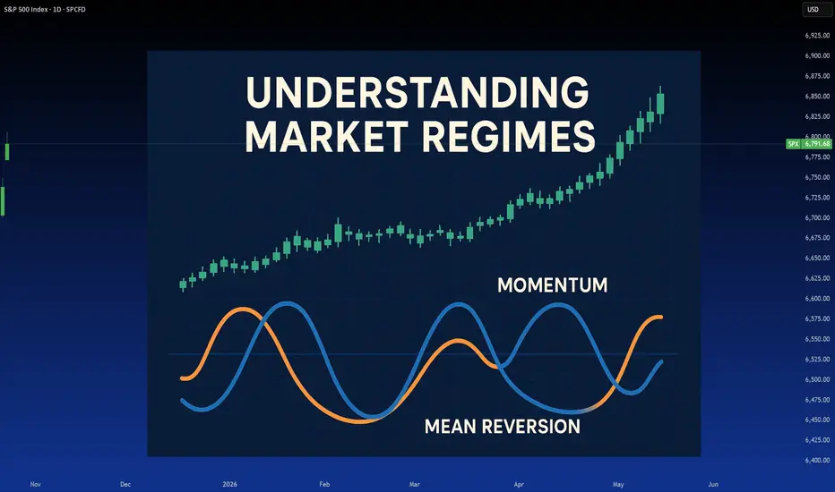
$FARTCOIN (DAILY): all-year long FALLING WEDGE, WAVE A on?SEED_WANDERIN_JIMZIP900:FARTCOIN is basically a BEAR MARKET coin and has been for longer nearly two months, it lost the 200 MA in August and retested twice in September, from below.
So, a DOWNTREND, all moving averages overhead and curving down, just hopeless. $380M marketcap coin, by the way, that was 7 times bigger last DECEMBER. Mad.
OBV profile has been compelling since the JULY local top, remained stable with multiple BULL divergences, it's been a theme.
That's why I'm watching this distaster of a DAILY chart for any reversal signs, we might be doing a negative ELLIOT'S WAVE count WAVE A targetting 54c.
DEAD cat bounce or not, there might be a short-term LONG setup at some point. On my WATCHLIST for sure, definitely not READY.
👽💙

BTC 4H ENG.My kids are scared; they got scared with the October 10th crash. Do you know when they stop being scared? When it goes up! I have my futures take profits at 117k; you're my target. I've had my entry pattern very clear, since I was at 106k. The red box indicates an ideal entry area, although you should already be inside.

$LINK (DAILY): GOLDEN POCKET support / 200 MA fightBIST:LINK on its WEEKLY chart: still a text-book BAT reversal intact, below the 50 MA, and just continuation to the downside. High selling volumes recently and essentially reverting back to its mean (200 MA on 1W at $12.8), although that's a long term chart.
We need a look on the DAILY to get a better idea if a reversal to the upside is an option soon.
1D chart is showing a fight to stay above a combo of crucial pivots:
1) 200 MA at $17.7, key moving average, for many traders, especially institutional: bear/bull boundary
2) horizontal support/former resistance $17.4
3) GOLDEN POCKET of the move that took the price from JUNE lows ($11) all the way up to the AUGUST top ($28).
OBV on the DAILY had two minor HIDDEN BULLISH divergences while the price was finding support in the pocket, that's interesting to see.
Holding the green 200 MA is the most important thing for now, no reversal yet, but if it was to remain a BULL MARKET asset, the BUYERS must step in immediately.
Close below the GOLDEN POCKET and we should see $14.6 and possibly $12.8 if that doesn't hold.
LONGS only above $19.5, I need to see a BULLISH market structure change to do anything here.
👽💙

ARE TESLA MARKET BULLS BECOMING WEAK?Tesla Analysis (Weekly Timeframe)
Tesla is currently completing its first cycle wave since inception. The market started printing a primary wave 5, which is an ending diagonal in January 2023. Primary wave 5 comprise of 5 3-wave intermediate waves 1,2,3,4 and price is now printing intermediate wave 5. Intermediate wave 5 started printing in March 2025, minor wave A terminated in May 2025 and minor wave B, a running flat terminated in July 2025. The market is now printing an impulse minor wave C to complete the last 3-wave intermediate wave 5 that will complete primary wave 5 that will complete cycle wave 1. Intermediate wave 5 may be truncated, i.e., it does not necessarily have to touch the medium-term bullish resistance line (upper trendline). From here we will see a major primary wave ABC correction that may begin in Q1 of 2026.
Short entries (1) @ 488.93
Short entries (2) @ 511.04
SL @ 533.15
TP @ 321.47
"The big money is not in the buying or selling - but in the waiting" Charlie Munger
#SabaliCapital
#TechnicalAnalysis

LINK - BULLISH SCENARIO BIST:LINK - price analysis 🍿
Almost the same PA as $DOGE.
Very neutral area on the monthly, big volatility on both side. Really hard to trade & find a direction on the short term.
A Monthly close above 18.00$ would be good for bulls regarding the tails + Kijun level ichimoku.
Bullish consolidation likely if it hold above 15.80$ daily basis.
Local key support:
16.70 - 16.55$ - 15.70$
Price seems to be moving inside this downtrend channel ; but 👇
Possible bullish setup: $
A breakout of downtrend would surely lead to a push toward 20.00$ or even 22.80$ to fill the gap! 📈
Weekly resistance: 19.55 - 20.50 -
Also, I Hope that's not a bearish H&S pattern (3rd chart) with a neckline around 20.00 - 20.30$, otherwise, big bearish move could happen. 👀

SOL: One More High… or Goodbye?The Solana bull run that started in December 2022 most likely finished in January 2025. It was a textbook five-wave impulse (extended iii, with i ≈ v). From Jan → Apr 2025 we saw the first leg down (A), and the rally Apr → Sep was merely a corrective (B) move; base case is C down toward $80–50. An alternative allows for one more pop within B (even a small over-throw), but downside resumes after.
Full cycle & proportions
Dec ’22 → Jan ’25: clean 1–2–3–4–5.
Wave 3 shows a classic extension.
Waves 1 and 5 are nearly equal in length.
The run from the bottom is roughly 30–35× (about +3,000%), which statistically argues for a meaningful mid-term correction.
Base correction targets from the whole impulse: 0.382–0.5 Fib → $80–50, aligning with monthly/quarterly imbalances (FVG).
What 2025 looked like
Jan → Apr: first downward leg — wave A.
Apr → Sep 18 (high ~$253): a double zigzag W–X–Y — typical wave B, not a new trend.
Alternative (expanded flat, EFL)
A: Jan → Apr 7 down.
B: Apr → Sep as (A); now forming (B); then (C) up (a minor higher high is possible).
After that, a larger C down into $80–50.
Why I think the rally is done (market context)
TOTAL and BTC likely trace end-phase bull structures (distribution/terminal patterns).
Volume profile on COINBASE:SOLUSD : the heaviest trading sits around $120–200 (HVN/POC) — classic distribution; price often moves below POC afterwards.
Price Action (weekly/monthly): $216–260 is a major resistance that launched the bear market back in Nov 2021. Repeated tests without a weekly/monthly hold above it argue against an immediate breakout.
Fundamentals in two lines
Why a correction now: cycle overextension, liquidity saturation near the top, sensitivity to DXY/real yields and risk-off in US indices.
Why the long-term case survives: high throughput, latency improvements (e.g., Firedancer), growing DeFi/stablecoin/consumer activity. After leverage clears, BINANCE:SOLUSDT historically recovers with high beta.
Levels & invalidation
Base (correction) holds until we get a weekly close > $260–270.
Downside waypoints: $150 → $120 → $95 → $80–50.
Invalidation: sustained hold above $270 with expanding volume — I’d concede an early start of (3) without a deep (2).
Bottom line. With high probability, SOL’s medium-term rally is over; we are in a corrective phase targeting $80–50. The long-term bullish story can resume later — but first the market likely needs to deflate.

Bitcoin playing games at critical levelsBTC is clearly causing the market to capitulate over time. Price capitulation has already been achieved for the most part. The current sideways chop causes many traders to lose focus and exhaust their patience. This is what the market wants. There are some good signs of support at the current H1 structure, but let your guard down, this PA is CRAZY.

GBPAUD Trading Opportunity! BUY!
My dear friends,
Please, find my technical outlook for GBPAUD below:
The price is coiling around a solid key level - 2.0436
Bias - Bullish
Technical Indicators: Pivot Points Low anticipates a potential price reversal.
Super trend shows a clear buy, giving a perfect indicators' convergence.
Goal - 2.0524
About Used Indicators:
The pivot point itself is simply the average of the high, low and closing prices from the previous trading day.
Disclosure: I am part of Trade Nation's Influencer program and receive a monthly fee for using their TradingView charts in my analysis.
———————————
WISH YOU ALL LUCK

BONK: ALTsummers darling is dumping.BONK – One of the First Runner of #ALTSummer
BONK was one of the first tokens to blast off this summer, setting the pace for early alt momentum. It completed what looks like a clean five-wave impulse up, but now we’re seeing the market digest that move.
If the structure were still strongly bullish, we’d expect a simple internal retracement into the summer impulse before continuation. Instead, the current price action is drifting lower and looks ready to sweep the origin of that move. That tells us this may be more than just a pullback.
On the hard right edge, the structure is giving off triangle vibes. The range is tightening, volume is contracting, and the swings are overlapping. In Elliott Wave terms, a triangle is often the final pattern before the last move of a sequence. It’s the market coiling up before making its decision.
If this forms and finishes as a triangle, we can use it to anchor the count. A clean thrust and sweep of the pivot could trigger short-term upside and possibly close out the current leg. From there, the key question becomes whether that push is the start of something new or simply the last gasp before one more low.
For now, I’m watching how BONK handles this pattern. If it holds and breaks above the triangle invalidation, that would confirm a short-term bullish response. If it completes and breaks lower, the summer impulse is likely complete, and the next real opportunity will come from the base that forms afterward.
Trade safe, trade clarity.
TonyTalon
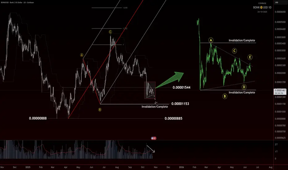
$ALUMINIUM (DAILY): LONG position in-play, DOUBLE BREAKOUT onOpened this PEPPERSTONE:ALUMINIUM LONG position this week as the price started closing above the $2800 mark that I had been waiting for.
Essentially a mega strong DOUBLE BREAKOUT ongoing, the RECTANGLE and the TRIANGLE, targetting $3165 and $3375, respectively.
Stop loss when #aluminium loses its breakout point, simple trade, this one.
This WAVE could either be number 3 or 5, but regardless, the momentum has been great, confirmed by a few HIDDEN BULLISH RSI divergences in a row.
Commodities season. Crypto sucks this quarter, open your minds.
👽💙